Unveiling The Power Of Beta Priors In Likelihood Maps: A Comprehensive Guide

Unveiling the Power of Beta Priors in Likelihood Maps: A Comprehensive Guide

Related Articles: Unveiling the Power of Beta Priors in Likelihood Maps: A Comprehensive Guide

Introduction

With enthusiasm, let’s navigate through the intriguing topic related to Unveiling the Power of Beta Priors in Likelihood Maps: A Comprehensive Guide. Let’s weave interesting information and offer fresh perspectives to the readers.

Unveiling the Power of Beta Priors in Likelihood Maps: A Comprehensive Guide

In the realm of Bayesian statistics, the concept of prior distributions plays a pivotal role in shaping our inferences. Among these priors, the Beta distribution stands out as a versatile tool for modeling probabilities and proportions, particularly when applied to likelihood maps. This article delves into the intricacies of Beta priors within the context of likelihood maps, highlighting their significance and practical applications in various domains.

Understanding Likelihood Maps and Beta Priors

A likelihood map is a visual representation of the probability of an event occurring across a defined space. It serves as a powerful tool for visualizing uncertainty and identifying areas of high or low probability. In the context of Bayesian analysis, likelihood maps are often constructed by combining prior knowledge with observed data.

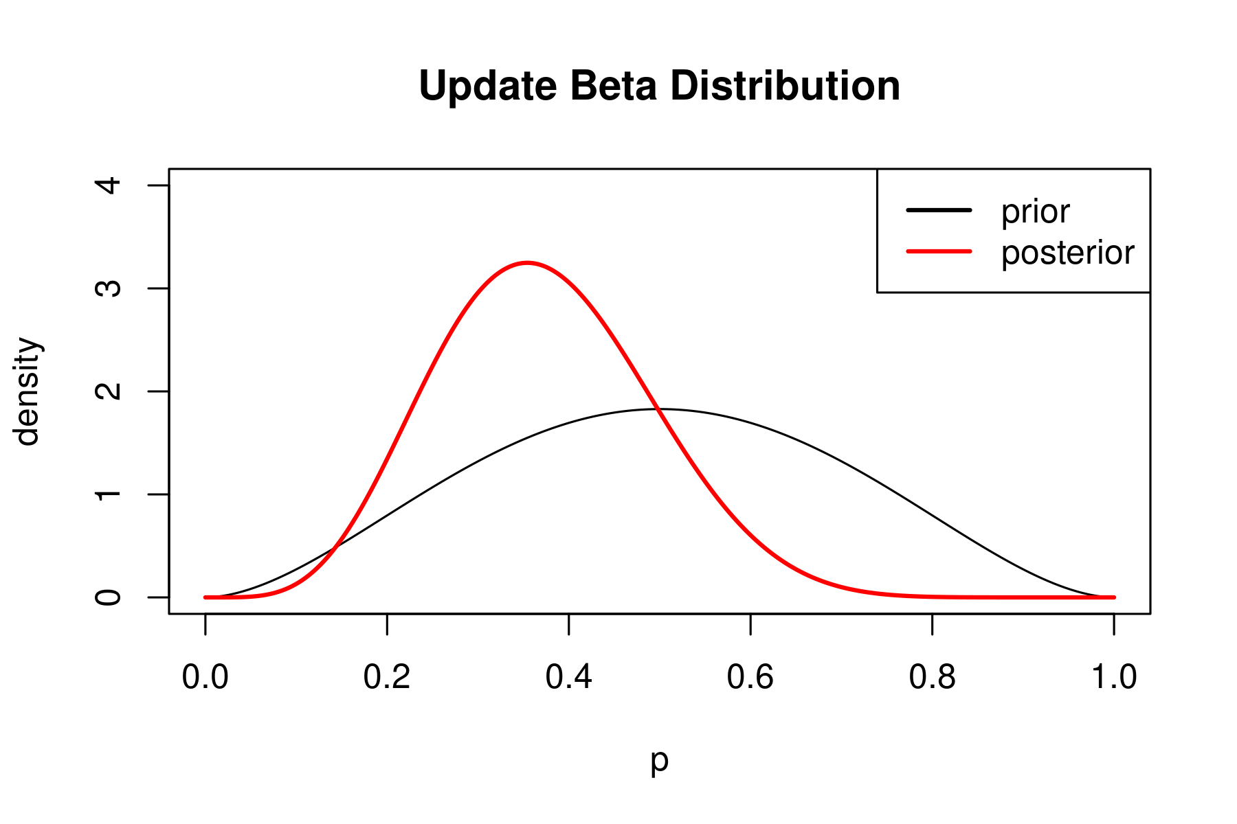
The Beta distribution, a continuous probability distribution defined over the interval [0, 1], emerges as a natural choice for representing prior beliefs about probabilities or proportions. Its two parameters, denoted as α and β, control the shape of the distribution, allowing for flexible modeling of various prior assumptions.

The Advantages of Beta Priors in Likelihood Maps

1. Intuitive Interpretation: Beta priors are inherently interpretable, with parameters α and β directly reflecting the prior belief about the probability of an event. For instance, a Beta distribution with α = 2 and β = 1 suggests a prior belief that the probability of the event is slightly more likely than not.

2. Flexibility and Adaptability: The Beta distribution exhibits remarkable flexibility, capable of representing a wide range of prior beliefs. From strong prior convictions to vague assumptions, the Beta prior can be tailored to reflect the available information.

3. Conjugate Prior: The Beta distribution is a conjugate prior for the Bernoulli distribution, meaning that the posterior distribution, obtained after incorporating observed data, also follows a Beta distribution. This property simplifies calculations and facilitates efficient inference.

Applications of Beta Priors in Likelihood Maps

The combination of Beta priors and likelihood maps finds applications in diverse fields:

• Medical Imaging: In medical imaging, Beta priors can be employed to model the probability of tumor presence or disease severity based on observed image features. This approach aids in diagnosis and treatment planning.

• Machine Learning: Within machine learning, Beta priors are used in probabilistic models such as Bayesian logistic regression, where they serve to regularize model parameters and improve generalization performance.

• Natural Language Processing: In natural language processing, Beta priors can model the probability of word occurrence in different contexts, leading to improved language modeling and text generation.

• Finance and Economics: Beta priors are valuable in financial modeling, helping to estimate probabilities of default or market volatility. They also play a crucial role in economic forecasting and risk assessment.

Illustrative Example: Modeling Disease Prevalence

Consider a scenario where we want to estimate the prevalence of a specific disease in a population. We have access to a dataset containing health records of individuals, where each record indicates the presence or absence of the disease.

Using a likelihood map, we can visualize the probability of disease prevalence across different geographical regions. By incorporating a Beta prior, we can introduce prior knowledge about the disease prevalence based on previous studies or expert opinions. This prior information can guide the estimation process and improve the accuracy of the resulting map.

Python Implementation

Python’s rich ecosystem of libraries provides powerful tools for working with Beta priors and likelihood maps. Libraries like scipy and numpy offer functions for manipulating Beta distributions and generating likelihood maps.

Code Snippet:

import numpy as np
from scipy.stats import beta

# Define prior parameters
alpha = 2
beta = 1

# Generate a grid of probabilities
probs = np.linspace(0, 1, 100)

# Calculate the prior distribution
prior = beta.pdf(probs, alpha, beta)

# Visualize the prior distribution
plt.plot(probs, prior)
plt.xlabel("Probability")
plt.ylabel("Prior Density")
plt.title("Beta Prior Distribution")
plt.show()

FAQs

Q: How do I choose the appropriate values for α and β in the Beta prior?

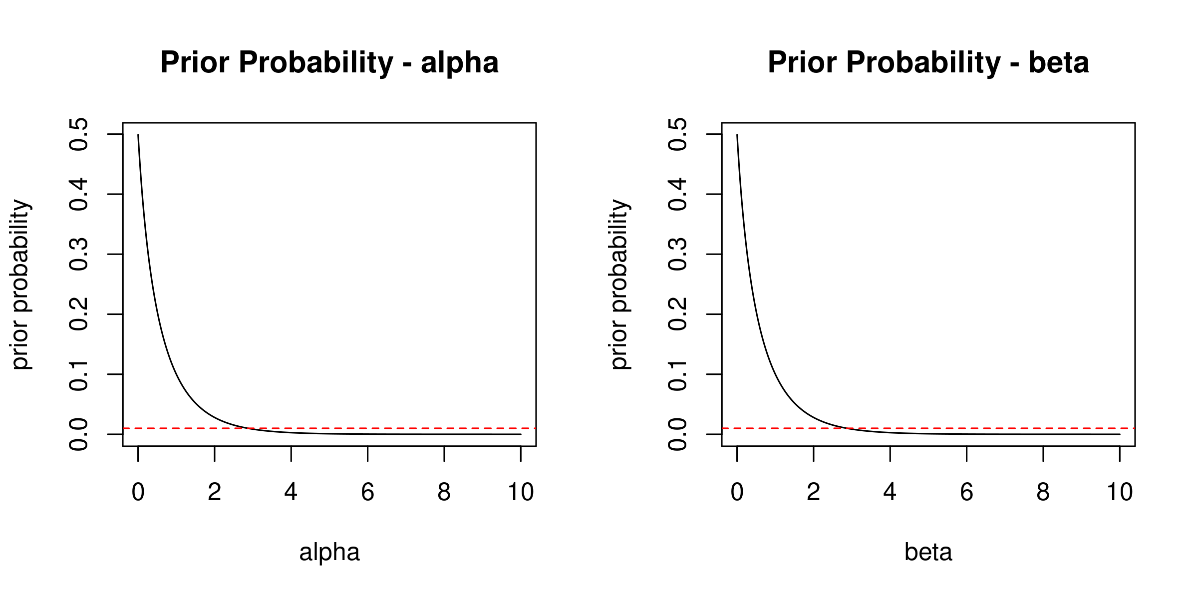
A: The choice of α and β depends on the available prior knowledge. If there is strong prior information, α and β can be set to reflect this knowledge. If prior information is vague, α and β can be set to low values, indicating a non-informative prior.

Q: How do I incorporate observed data into the likelihood map?

A: Observed data is incorporated through the likelihood function. The likelihood function represents the probability of observing the data given different values of the parameter of interest. The posterior distribution is then obtained by combining the prior distribution with the likelihood function.

Q: What are the limitations of using Beta priors in likelihood maps?

A: While Beta priors offer significant advantages, they are not without limitations. One limitation is that they assume a unimodal distribution, which may not be appropriate for all scenarios. Additionally, the choice of α and β can influence the results, and careful consideration is required to ensure that the prior reflects the available knowledge accurately.

Tips

• Explore different prior distributions: While the Beta distribution is a popular choice, other priors may be more appropriate depending on the specific application.

• Utilize sensitivity analysis: Perform sensitivity analysis to assess the impact of different prior choices on the results.

• Visualize the results: Visualizing the likelihood map and the posterior distribution helps in understanding the impact of the prior and the observed data.

Conclusion

Beta priors, when integrated with likelihood maps, provide a powerful framework for incorporating prior knowledge into Bayesian inference. Their flexibility, interpretability, and conjugacy make them valuable tools in a wide range of applications. By carefully considering the choice of prior parameters and incorporating observed data, researchers and practitioners can leverage the power of Beta priors to gain deeper insights from data and make more informed decisions.

Closure

Thus, we hope this article has provided valuable insights into Unveiling the Power of Beta Priors in Likelihood Maps: A Comprehensive Guide. We thank you for taking the time to read this article. See you in our next article!